

Contents
Tags
Share:
1. Change Between Multiple Excel Documents (and general programs)
Working on several spreadsheets at once can be difficult, especially if you only have one screen; you could end up working on the completely wrong sheet, wasting valuable time. Using Alt + Tab will allow you to easily shift between different files freely. This function is also applicable to other files or programs open on your Windows PC.

2. Add More Than One New Row or Column
You might know how to add a new row or column, but if you are looking to add more than one, rather than repeating the action multiple times, do it all at once. The best way is to drag and select the number of rows or columns (X is two or more) if you want to add X rows or columns above or left. Right-click the highlighted rows or columns and choose Insert from the drop-down menu. New rows will be inserted above the row or to the left of the column you first selected.

3. Make Life Easier, Add Some Filters
When you’re looking at large data sets, chances are you don’t need, or want to be looking at every single row at the same time – too confusing for the brain. Sometimes, you only want to look at data that fits certain criteria. That’s where filters come in.
Filters allow you to reduce your data, allowing you to only look at certain rows at a time. In Excel, a filter can be added to each column in your data and from there, you can then choose which cells you’d like to see.
Add a filter by clicking the Data tab and selecting “Filter”, clicking the arrow next to the column headers, and you’ll be able to choose whether you want your data to be organised in ascending or descending order, as well as which specific rows you want to show.
If I only want to see the employees in Sales, by selecting the Sales filter, the other rows disappear. Easy!
4. Remove Duplicates
Larger data sets tend to have duplicate content. You may have a list of multiple contacts in a company and only want to see the number of companies you have. In situations like this, removing the duplicates comes in quite handy.
To remove your duplicates, highlight the row or column that you want to remove duplicates from. Then, go to the Data tab, and select “Remove Duplicates”. A pop-up will appear to ask if you want to “Expand the selection” or “Continue with the current selection” this example, you want to stick to the data you have selected. Select “Remove Duplicates” and “OK”, then BAM, no more duplicates.
5. Text to Columns
What if you want to split out information that’s in one cell into two different cells? For example, maybe you want to pull out someone’s company name from their email address. Or perhaps you want to separate someone’s full name into a first and last name for your email marketing templates. Luckily, both options are possible and pretty easy to get to grips with.
Let’s take a look at how to separate someone’s full name into first and last name, this is something I have to do a lot of when creating marketing materials. First, highlight the column that you want to split up. Next, go to the Data tab and select “Text to Columns.” A module will appear with additional information.
First, you need to select either “Delimited” or “Fixed Width.”
- “Delimited” means you wish to break up the column based on characters such as commas, spaces, or tabs.
- “Fixed Width” means you want to select the exact location on all the columns where you want the split to occur.
For this example, we should select “Delimited” so we can divide the full name into first name and last name.
Next, we need to choose our Delimiters. This could be a range of things from tabs to semicolons or a space, (this could also be the “@” sign used in an email address.) In this example, it makes sense to choose the space! Then, press “Next” (this page will allow you to select Advanced Formats if you choose to). When you’re done, click “Finish.” Boom, you’ve just saved yourself some serious time!

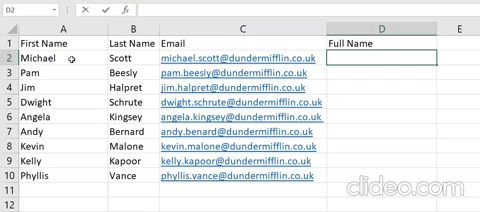
6. Combine cells using “&”
Let’s flip that like a pancake and combine cells with different data into one cell, by using the “&” sign in your function!
The formula with variables from our example below: =A2&” “&B2
Let’s say we now want to combine first names and last names into full names in a single column. To do this, select the blank cell you want the full name to appear in. Then, we need to highlight one cell that contains a first name, type in an “&” sign, and then highlight a cell with the corresponding last name.
But hold on, you’re not finished there. If all you type in is =A2&B2, then there will not be a space between the person’s first name and last name. To add that necessary space, use the function =A2&” “&B2. The quotation marks around the space tell Excel to put a gap in between the first and last names.
To make this true for multiple rows, simply drag the corner of that first cell downward as shown in the example, or double-click the cell.
7. Quick Maths
Excel is somewhat known for its complex calculating abilities, but before you move on to the difficult stuff, make sure you master the basics first! Excel can help you do simple arithmetic like adding, subtracting, multiplying, or dividing your data.
- To add, use the + sign.
- To subtract, use the – sign.
- To multiply, use the * sign.
- To divide, use the / sign.

You can also create averages for a set of numbers, using the formula =AVERAGE(Cell Range). If you want to sum up a column of numbers, you can use the formula =SUM(Cell Range).
8. Conditional Formatting Formula (Fancy Colour Coding)
Colour coding always make data easier to understand, which is, in a sense, what Conditional formatting is. It allows you to change a cell’s colour based on the information within the cell. For example, if you want to note certain numbers that are above average or in the top 25% of the data in your spreadsheet, you can do that. If you want to colour-code commonalities between different rows in Excel, you can. This allows you to see the information that is important to you faster.
To get started, highlight the group of cells you want to use conditional formatting on. Then, choose “Conditional Formatting” from the Home menu and select your logic from the dropdown. Note how you can also create your own rule if you want something different. A window will pop up that prompts you to provide more information about your formatting rule. Select “OK” when you’re done, and you should see your results automatically appear. Ta-da!
9. What “IF Statement”?
Sometimes, we don’t want to count the number of times a value appears. Instead, we want to input different information into a cell if there is a corresponding cell with that information.
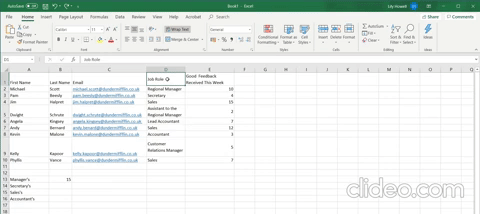
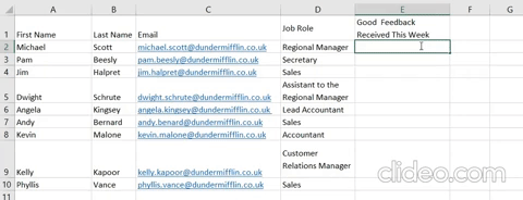
For example, in the situation below, I want to add three “good feedback” points to everyone in the Sales team. Instead of manually typing in 3’s next to each Sale’s person’s name (which could take forever), I can use the IF THEN Excel formula to say that if the employee is in Sales, then they should get three points.
The formula: IF(logical_test, value_if_true, value of false)
Example Shown Below: =IF(D2=”Sales”,”3″,”0″)
In general terms, the formula would be IF(Logical Test, value of true, value of false). Let’s check out what each of these variables means.
- Logical_Test: The logical test is the “IF” part of the statement. In this case, the logic is D2=”Sales” because we want to make sure that the cell corresponding with the employee says “Sales.” Make sure to put Sales in quotation marks here.
- Value_if_True: This is what we want the cell to show if the value is true. In this case, we want the cell to show “3” to indicate that the staff were awarded the 3 points. Only use quotation marks if you want the result to be text instead of a number.
- Value_if_False: This is what we want the cell to show if the value is false. In this case, for any employee not in Sales, we want the cell to show “0” to show 0 points. Only use quotation marks if you want the result to be text instead of a number.
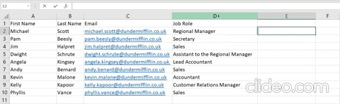
10. See Trends With The COUNTIF Function
With the COUNTIF function, Excel can count the number of times a word or number appears in any range of cells, relieving you of tedious manual work that could take more time than you have.
For example, let’s say I want to count the number of times the word “Sales” appears in my data set.
The formula: =COUNTIF(range, criteria)
The formula with variables from our example below: =COUNTIF(D:D,”Sales”)
In this formula, there are several variables:
- Range: The range that we want the formula to cover. In this case, since we’re only focusing on one column, we use “D:D” to indicate that the first and last column are both D. If I were looking at columns C and D, I would use “C:D.”
- Criteria: Whatever number or piece of text you want Excel to count. Only use quotation marks if you want the result to be text instead of a number. In our example, the criterion is “Sales.”
Simply typing in the COUNTIF formula in any cell and pressing “Enter” will show me how many times the word “Sales” appears in the dataset.
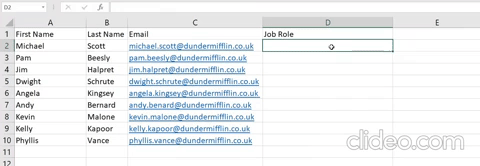
11. Merge Data With The VLOOKUP Function
This one’s a biggie and something we’ve probably all come across! This is for when you have two sets of data on two different spreadsheets and you want to combine them into a single spreadsheet.
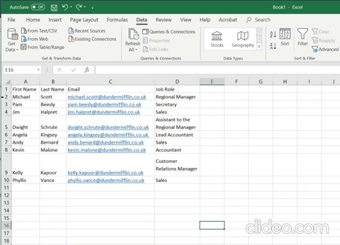
For example, you might have a list of people’s names next to their email addresses in one spreadsheet, and a list of those same people’s email addresses next to their company names in the other — but you want the names, email addresses, and company names of those people to appear in one place.
Read carefully because it may take you a few attempts to get this one…
The formula we’re using is: =VLOOKUP(lookup value, table array, column number, [range lookup])
My example formula is: =VLOOKUP(C2,Sheet2!A:B,2,FALSE)
In this formula, there are several variables. The following is true when you want to combine the information in Sheet 1 and Sheet 2, onto Sheet 1.
- Lookup Value: This is the identical value you have in both spreadsheets. Choose the first value in your first spreadsheet. In the example that follows, this means the first email address on the list, or cell 2 (C2).
- Table Array: The range of columns on Sheet 2 you’re going to pull your data from, including the column of data identical to your lookup value (in this example, email addresses) in Sheet 1 as well as the column of data you’re trying to copy to Sheet 1. In our example, this is “Sheet2!A:B.” “A” means Column A in Sheet 2, which is the column in Sheet 2 where the data identical to our lookup value (email) in Sheet 1 is listed. The “B” means Column B, which contains the information that’s only available in Sheet 2 that you want to translate to Sheet 1. That was a lot, are you still with me?
- Column Number: The range of columns you just indicated tells Excel which column the new data you want to copy to Sheet 1 is located in. In our example, this would be the column in “Job Role” is located in. “Job Role” is the second column in our range of columns (table array), so our column number is 2.
- Range Lookup: Use FALSE to ensure you pull in only exact value matches.
In the example below, Sheet 1 and Sheet 2 contain lists describing different information about the same people, and the common thread between the two is their email addresses. What if we want to combine both datasets so that all the house information from Sheet 2 translates over to Sheet 1? If you apply the logic you learnt above, you can do just that!
As technology evolves, so does the functionality of Excel. Here's a quick overview of some of the latest tools and features:
1. Leveraging AI in Excel - Explore how Excel is incorporating AI tools for enhanced data analysis.
- Excel Blog | Microsoft Community Hub
2. Excel on the Web - Discover how using Excel in a web-based format can facilitate real-time collaboration.
- How to Use Excel Like a Pro
3. Advanced Formulas - Dive into the latest functions that can better manage your data.
- 50 Top Microsoft Excel Tips
So there we go; hopefully, you picked up a thing or two along the way that will help your Excel work less time-consuming! Learning how to get the best out of the software you are using will add real value to the work you produce in a fraction of the time.